The problem is that I often need to run a lot of simulations on the same circuit. For example, a bandgap, I want to run DC, run loopgain, and sometimes add Chopper and run tran. This creates a problem: I need to create quite a bit of ADE state (because the author's company has an ocean-like GUI, each simulation, such as PVT variation or Monte Carlo, requires a corresponding ADE state).
Because the author is also willing to save trouble. So a colleague taught the following method to avoid the setting of the new ADE.
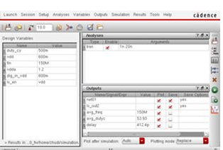
1st, I have a simulation.
2nd, I want to vary the simulation conditions:
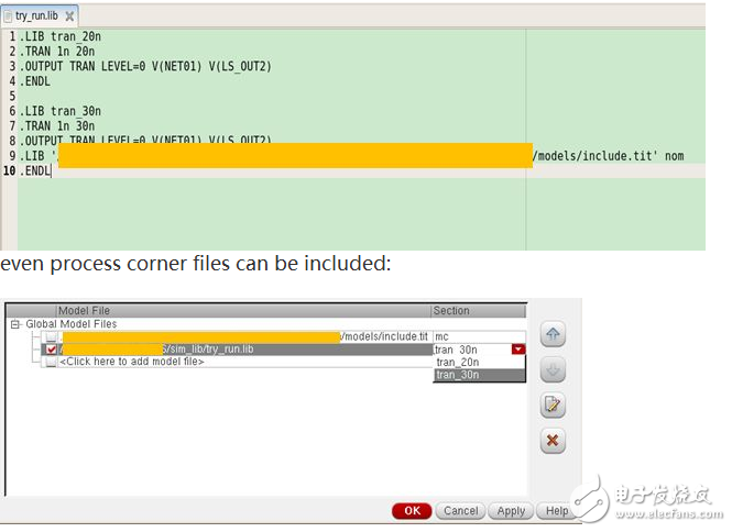
I create a file:
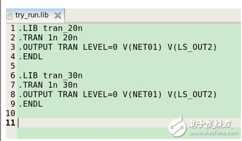
3rd, I add the above file in my libs.
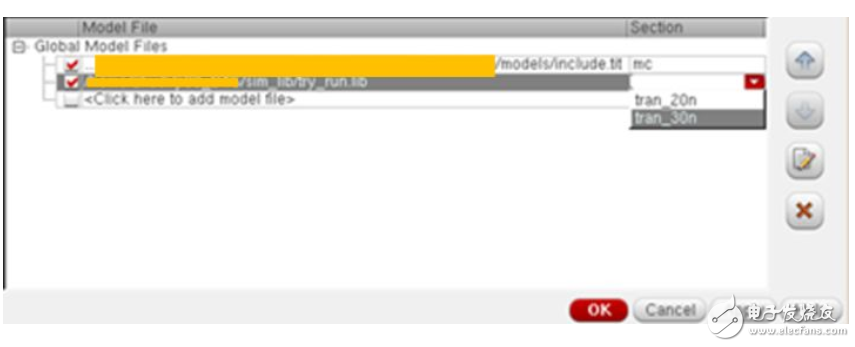
4th, I choose the required condition, and run the simulations:
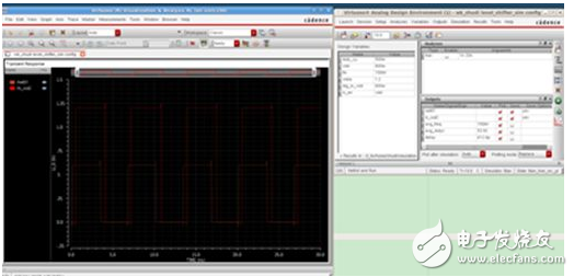
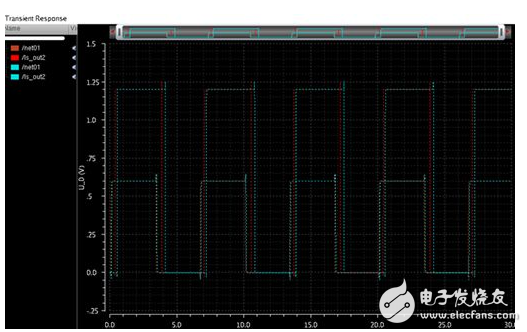
As you can see, in the appearance interface, the simulation length is 20ns, but the output waveform is 30ns, because I chose my LIBS 30ns. (Remember to disable the original check in ADE)
Try it! ! !
By selecting the required library file, you can run many different conditions in the same ADE state.
Or you can create a file to control the library.
Ghosts can be run with commands without having to set them in the GUI.
Then, I tried again and could not nest the "lib" function, such as nesting the model file lib in my lib (that is, the text file just written), and then found that it is ok.
I modified the last word of the technical file, "Fast" and "Title", and you can see the results are different.
Therefore, you can create 1 file to cover all the conditions you want to check.
Please refer to the following page, you can plot the parameters such as vth, gm (the author often does this when doing bandgap, and then can get parameters such as beta, Nf):
How to save DC operating point â€TM parameters in Cadence MOSFET
This will describe how to save the DC parameters of the MOSFET in Cadence.
Set up a circuit as shown below.
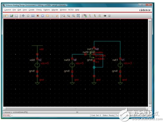
Record the instance name of the transistor (N0 is the instance name of the transistor of the above circuit).
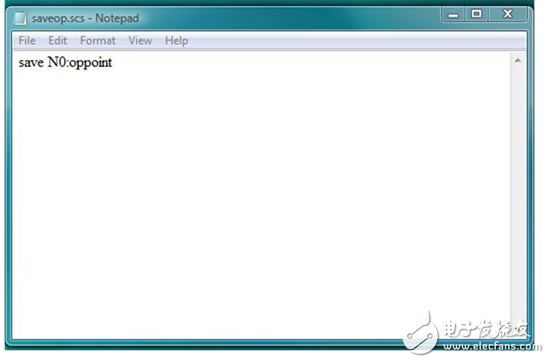
Open a text file and add the save N0 ": party specified "save as" saveop. South Sea" file, as shown below

Next, click on the simulation environment simulator launched by "Start → ADE L".
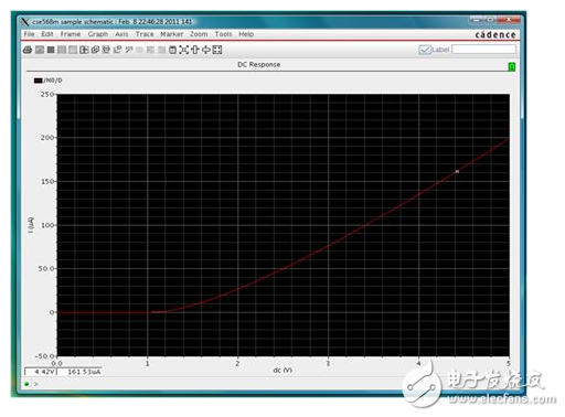
In the simulator, select DC analysis and scan the voltage from 0 to 5V.
Select the drain current on the schematic as the output of the plot.
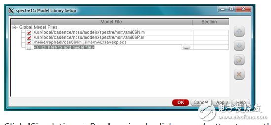
Select "Settings → Model Library" and load saveop.scs as shown below.
Click "Simulate → Run" or click the green button to run the simulation.
The output of Cadence will look like this:
On the emulator, click on "Tools → Results Click on Browser". Also, click on "Tools → Browser" in the output graph.
Browse to the PSF file associated with the simulation.
Select "DC" to see the transistor N0 parameters as shown below.
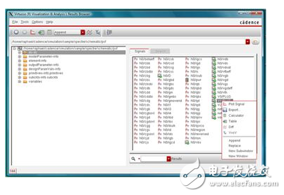
Right click on the story in the list, put any parameters, or export the value (s) to a file.
Incremental encoders provide speed, direction and relative position feedback by generating a stream of binary pulses proportional to the rotation of a motor or driven shaft. Lander offers both optical and magnetic incremental encoders in 4 mounting options: shafted with coupling, hollow-shaft, hub-shaft or bearingless. Single channel incremental encoders can measure speed which dual channel or quadrature encoders (AB) can interpret direction based on the phase relationship between the 2 channels. Indexed quadrature encoders (ABZ) are also available for homing location are startup.
Incremental Encoder,6Mm Solid Shaft Encoder,Hollow Rotary Encoder,Elevator Door Encoder
Jilin Lander Intelligent Technology Co., Ltd , https://www.landerintelligent.com